Mapping toolbox in MATLAB for easily plotting and analysis

Mapping Toolbox™ provides algorithms and functions for transforming geographic data and creating map displays. You can visualize your data in a geographic context, build map displays from more than 60 map projections, and transform data from a variety of sources into a consistent geographic coordinate system.

As we all know, MATLAB provides a lot of toolboxes like Statistics and Machine Learning Toolbox, Signal Processing Toolbox™, Mapping Toolbox™ e.g. These toolboxes have many algorithms and functions for ease of our daily work and study. This article provides an example using MATLAB Mobile and Mapping toolbox for plotting and analyzing the walk pace data.

Requirements

• MATLAB mobile
• Mapping toolbox (MATLAB)

Optional

• Google Map API
• Statistics and Machine Learning Toolbox (MATLAB)

Acquisition of data

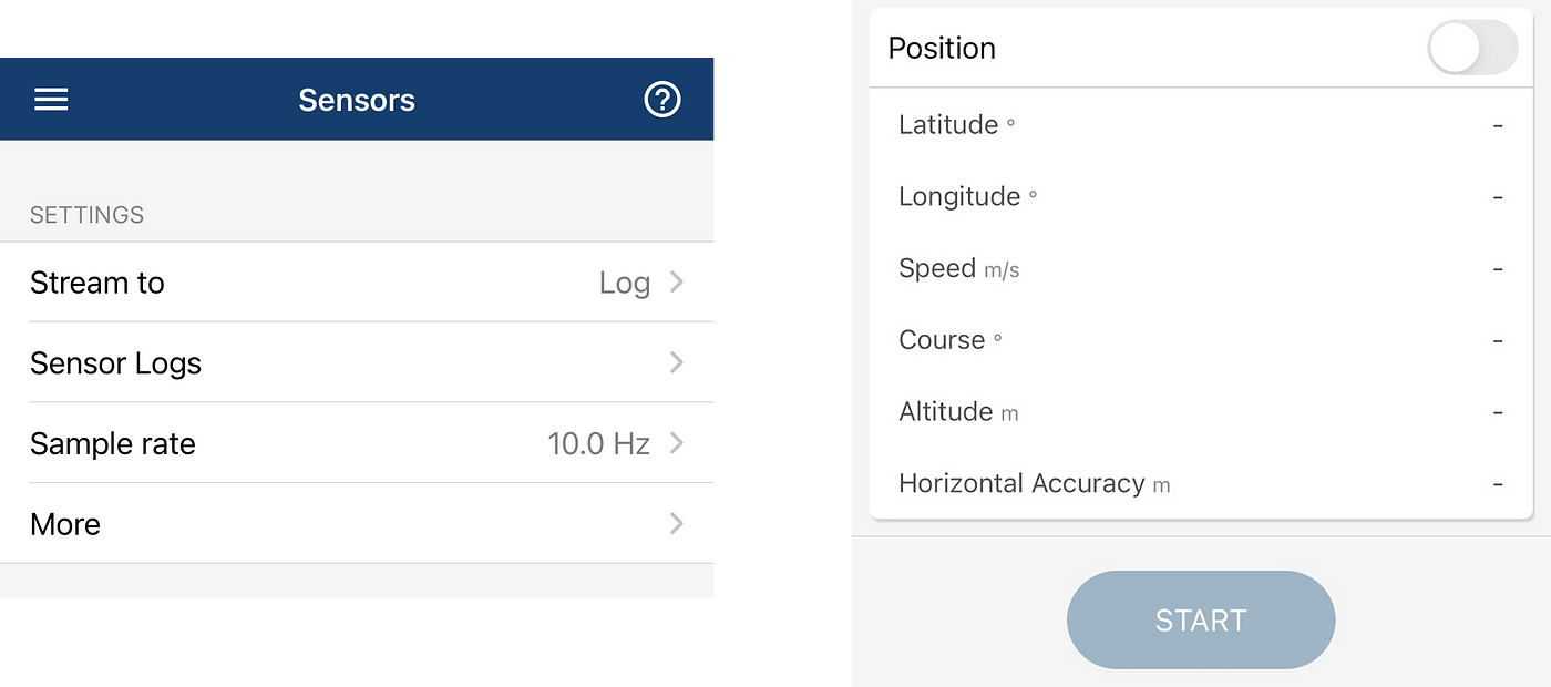
The MATLAB Mobile app provides a function named Sensors, including Acceleration, Magnetic Field, Orientation, Angular, and Position. You can select the most interesting data. Here I use the Position selection. The parameters are as below：

The data collected was like this:

Plot the data

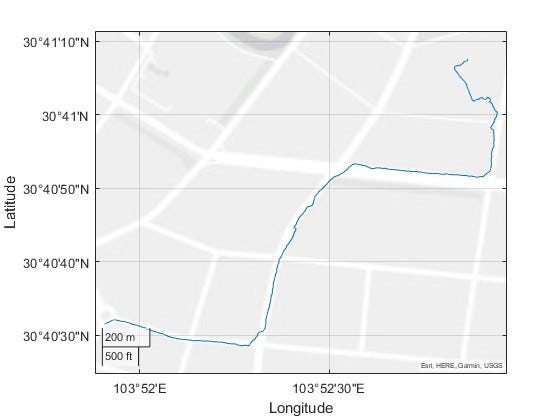
geoplot is the function for plotting lines in geographic coordinates. The syntax is like this geoplot(lat, lon).

Mapping Toolbox™ extends the functionality of the _geoplot_ (MATLAB®) function. It adds support for displaying points, lines, and polygons with coordinates in any supported geographic or projected coordinate reference system (CRS). For the _geoplot_ (Mapping Toolbox) page, see [_geoplot_](https://www.mathworks.com/help/map/ref/geopointshape.geoplot.html) (Mapping Toolbox).

So, we call the geoplot function:

geoplot(Position.latitude,Position.longitude)

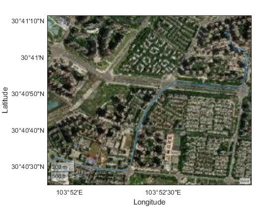
We can also change the base map using geobasemap, the types include streets, satellite e.g.

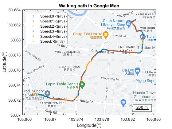
If you want to use the Google Map, a Google Map API is needed.

geobasemap satellite

Statistical Analysis

We can use the speed for grouping the data. Here I set 6 groups, which divided by speed.

When plotting the pace data, we can summarize the relationship between speed and road conditions, and traffic lights.

% Classification of the speed
speed = Position.speed;
speedInterval = strings(length(speed),1);  % String
for i = 1:length(speed)
    if speed(i,1) >= 0 && speed(i,1) < 1
        speedInterval(i,1) = 'Speed:0~1(m/s)';
    elseif speed(i,1) >= 1 && speed(i,1) < 2
        speedInterval(i,1) = 'Speed:1~2(m/s)';
    elseif speed(i,1) >= 2 && speed(i,1) < 3
        speedInterval(i,1) = 'Speed:2~3(m/s)';
    elseif speed(i,1) >= 3 && speed(i,1) < 4
        speedInterval(i,1) = 'Speed:3~4(m/s)';
    elseif speed(i,1) >= 4 && speed(i,1) < 5
        speedInterval(i,1) = 'Speed:4~5(m/s)';
    else 
        speedInterval(i,1) = 'Speed:>5(m/s)';
    end
end
hold on;
color = lines(3);
gscatter(lng,lat,speedInterval,color(1:3,:));  % gscatter:Scatter plot by group
legend('Location','northwest');
title('Walking path in Google Map');
xlabel('Longitude(°)');
ylabel('Latitude(°)');